Production Analysis Questions and Answers AP Inter 1st Year Economics Chapter 4

AP Inter 1st Year Economics 4th Lesson Production Analysis Questions and Answers

Essay Questions

Write an essay on the following questions.

Question 1.
Explain the law of variable proportion with the help of a diagram.
Answer:
An important law relating to production (producers) is the law of variable proportions. The law states that when a business firm increases one variable factor, keeping the other fixed factors constant, the increase in output is not proportional or not equal to the increase in the quantity of variable input. This law is also known as Law of diminishing returns and was introduced by Prof. Marshall. The law mostly applies in agricultural sector and is applicable only in the short run.

Definition : Marshall has defined the law as below.

“An increase in the amount of labour and capital applied in the cultivation of land causes, in general, a less than proportionate increase in the amount of output raised, unless it happens to coincide with an improvement in the arts of agriculture”.

Assumptions: The law is based on the following assumptions.

1. It is possible to change some inputs, keeping other factors/inputs constant to increase production.
2. State of technology or methods of production remain constant.
3. All units of variable inputs (labour) are homogeneous.
4. The firm operates in the short period or short run.

The law can be explained with the help of the following table.

Fixed Factor (Land in Acres)	Variable Factor	Total Product	Average Product	Marginal Product	Stages of the law operates
5	1	50	50	50	Stage I (Increasing Returns)
5	2	120	60	70
5	3	180	60	60
5	4	200	50	20	Stage II (Diminishing Returns)
5	5	200	40	0
5	6	180	30	– 20	Stage III (Negative Returns)
5	7	140	20	– 40

In the table 4.1, it is shown that one input (labour) increases while other factors remain constant results, the proportion varies. Hence, this is known as the law of variable proportions. The table shows the total, average and marginal products change as a result of the change in the proportion between the variable input (labour) and the fixed inputs (land and capital): The production process is categorized into 3 distinct stages.

Graphical Illustration of the Law:

This is explained in the following diagram.

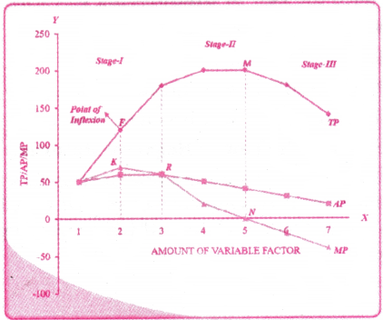
Explanation of the graph:

In the above graph (fig), the number of variable factor (Laborers) is shown on the OX-axis and Output (TP, AP and MP) is shown on OY-axis. According to this law, the production behavior can be studied in three stages as identified in the above graph. They are :

1. First Stage : In this stage.

• The Total Product )TP) curve increases at an increasing rate upto the ponit ‘F’ (Point of Inflexion, where MP is maximum) and then increases at a diminishing rate.
• The Average Prodcuct (AP) cuve goes on rising throughout the stage and became constant.
• The Marginal Product (MP) curve first rises and then falls after reaching its maximum, (as shown by point ‘K’ in the figure).
• The first stage ends when the Average Product is equal to the Marginal Product (AP = MP) and AP is maximum (or) constant.
• This stage is called as the Law of Increasing Returns.

Reasons : The main reasons for the operation of this stage of production are (a) indivisability of fixed factor, (b) Division of labour and Specialization.

2. Second Stage : In this stage.

• The total Product (TP) curve increass at diminishing rate and reaches its maximum and constant at POint ‘M’ (Saturation Point).
• The Aveage Product (AP) curve starts to fall after reaching its maximum (at AP=MP)
• The Marginal Product (MP) curve continuously falls and becomes zero at the point of saturation i.e., at point ‘M’ (Here, the slope of Total product is zero at point ‘M’).
• Second stage ends, where total product is at its maximum and marginal product is zero.
• This stage is called the Law of Diminishing Returns.

3. Third Stage (Law of Negative Returns): In this stage,

• The total Product (TP) curve falls.
• The Average Product (AP) curve continues to fall.
• The marginal Product (MP) curve becomes negative.
• This stage is called as the Law of Negative Returns.

Conclusion : In all three stages, the producer prefers to operate in stage – II. In this stage, the proper utilisation of resources is possible. The law of variable proportions is a very crucial cocnept which helps the producer to produce at an optimum level.

Importance of Law :

1. The law helps the business firms / producers to determine the optimum quantities of variable inputs.
2. The law helps the producers in determining the proportion between fixed input and variable input.
3. The law is also useful in the rational utilisation of scarce inputs/resources so as to minimise the cost of inputs (production) and to maximise profits/value of output.

Question 2.
Describe the law of return to scale with the help of a diagram.
Answer:
The Law of Returns to Scale, which applies in the long run, shows or explains the relationship between inputs and outputs in the long run. In the short run, to make changes in output, it is not possible to the producer to make changes in all the inputs. He can make changes only in variable inputs, by keeping constant all the fixed inputs. But in the long run, to increase or make changes in output, the producer can also make changes in fixed inputs.

The law of returns to scale explains, how output changes, in the long run, when there is an increase in the quantities of all inputs, both fixed and variable. When all the inputs are increased, the firm will experience three stages, namely the stage of increasing returns, followed by the stage of constant returns, further followed by the stage of decreasing returns.

The law of returns to scale can be explained with the help of table and diagram given below.

Returns to scale:

Units	Combination of Inputs	Total	Marginal	Stages
1.	10 Units of labour + 1 unit of capital	9	9	Increasing Returns to scale
2.	20 Units of labour + 2 units of capital	20	11
3.	30 Units of labour + 3 units of capital	32	12	Constant Returns to scale
4.	40 Units of labour + 4 units of capital	44	12
5.	50 Units of labour + 5 units of capital	55	11	Decreasing Returns to scale
6.	60 Units of labour + 6 units of capital

Question 3.
Distinguish between internal and external economies of scale and explain them.
Answer:
Nowadays, business firms have a tendency to produce goods on a large scale. They so because when they produce goods on a large scale, they get certain benefits known as economies of scale, also known as economies of large scale production.

Economies of large scale production are of 2 types. They are

1. Internal Economies,
2. External Economies.

1. Internal Economies: Internal economies are those economies or advantages which are available only to those firms which expand their size or take up production on a large scale.

2. External Economies : External economies are those economies or advantages which are enjoyed or available commonly to all the firms producing the same product, located at the same place.

Differences :

Internal Economies	External Economies
1) Internal economies are production based or scale or size based economies or benefits.	1) External economies are location based economies.
2) They are available only to those units which take up large scale production.	2) They are available even to those business units which may not produce on a large scale.
3) Internal economies are not common economies.	3) They are the common economies enjoyed by all units in a place.
4) These economies are visible in the form of saving or reduction in costs, larger output, improved quality of the goods, etc.	4) These economies are visible or reflected in the form of improved facilities, better infrastructure, tax concessions, etc.
5) Internal economies lead to business rivalry, severe competition, and feeling of enmity among business firms.	5) External economies lead to friendship, cooperation, the spirit of give and take, and sharing among business firms.
6) Internal economies, can be compared to the benefit or advantage of textbook reading available to only few textbook reading students in the class.	6) External economies can be compared to the benefit of expert teaching by a senior teacher, that is enjoyed by all the students assembled in the class.

Short Answer Questions

Write the answers briefly for the following questions.

Question 1.
Define the internal Economies ? Explain the types of Internal Economies.
Answer:
Internal Economies The word ‘Internal’ is used here to denote the limitation of these economies to the firm itself.

“Internal economies are those which are open to a single factory or a single firm independently of the action of other firms”. – Cairacross.

Types of Internal Economies

Technical Economies : Technical factors affect the returns to scale. Large firms will have more resources at their disposal. They will be able to install the most suitable machinery and adopt to advanced technology. As a result, they can lower cost of production.

Managerial Economies : With the increase in the scale of production, a firm can benefit from separate managerial departments or managers with specialisation. Each department is under the charge of an expert. A small firm can not afford this specialization. Experts are able to reduce the costs of production under their supervision.

Marketing Economies : As the scale of a firm is increased, it obtained economies of purchase and sale. Since the firm purchases on a large scale, it gets all the inputs at a cheaper rate compared to the smaller firms. Similarly wholesalers charge less for the sale of products to a large firm.

Financial Economies : A large firm will be able to reduce its costs of borrowing from the market. A bigger firm is better known to the financial institutions and the stock market. Therefore, a big firm has better access to credit and can borrow on more favourable terms. They can also attract investments.

Risk – bearing Economies : Large firms will be in a position to bear risks or avoid risks. They do so by diversifying output and markets. Therefore, loss in one good or in one market can be covered by profits in other goods and markets.

Question 2.
What are the factors that determine the supply ?
Answer:
Determinants of Supply :
a) Price of a Good : Other things being constant, the supply of a commodity mainly depends on its price. That means, supply of a commodity increases with an increase in its price and vice-versa.

b) Prices of Related Goods: If the price of a substitute good goes up, the producers will be induced to divert their resources to produce that substitute good and vice-versa. For example if the price of pulses increases while the price of rice remains constant, the farmer increases production of pulses and reduces production of rice.

c) Prices of factors of production: Increases in the price of one factor of production would lead to an increase in the cost of production. This results a fall in the profit margin. Consequently, the supply of the commodity will decline. The supply may increase if input prices fall.

d) State of Technology: Discoveries and innovations will help to increase the productivity of the factors and thus contribute to the raising of the supply of a commodity.

e) Government Policy: Imposition of heavy taxes on a commodity discourages its production, and as a result its supply diminishes. On the other hand, providing production subsidies will increase the production as a result its supply will increase.

f) Other factors: Means of transport and communication, goals of the producer, natural factors etc., are also other factors that determine supply of a commodity,

Question 3.
Define Isoquant ? Explain with the help of a graph.
Answer:
Consider a production function with two inputs labour and capital, An Isoquant is the set of all possible combinations of the two inputs that yield the same maximum possible level of output. Each isoquant represents a particular level of output and is labelled with that amount of output.

The shape of isoquant is Convex.

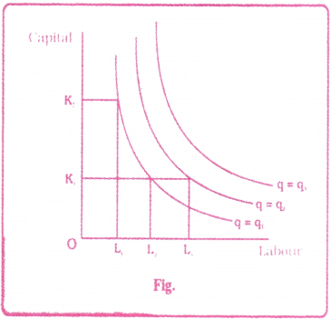
Isoquants are also known as equal product lines or producer indifference curves. The reason for slope of IQ curve is diminishing the Marginal Rate of Technical Substitution between two factors say labour & capital (MRTS_LK).

We place Labour (L) on the OX axis and Capital (K) on the OY axis. We have three isoquants for the three output levels, namely q = q₁, q = q₂ and q = q₃. Two input combinations (L₁, K₂) and (L₂, K₁) given us the same level of output q₁. If we fix capital at K₁ and increase labour to L₃, output increases and we reach a higher isoquant, q = q₂. When marginal products are positive, with greater amount of one input, the same level of output can be produced only using lesser amount of the other. Therefore, isoquants are negatively sloped.

Isoquants help the firms in finding the combination of inputs which minimizes the cost of production for a given output. This combination referred to as the “least-cost combination”.

Question 4.
The following table gives the total product schedule of labour. Find the corresponding average product and marginal product schedules of labour.

NL	TPL
0	0
1	15
2	38
3	54
4	40
5	35

Answer:
Average Product : Total Product divided by the number of units of labour (NL).
AP = TPL ÷ NL

Marginal Product : Change in Total Product when one more unit of labour is employed.
MP = ∆TPL

NL	TPL	AP
0	0	0 – 0
1	15	15 15 ( 15 – 15)
2	38	19 23 (38 – 15)
3	54	18 16 (54 – 38)
4	40	10 – 14 (40 – 54)
5	35	7 – 5 (35 – 40)

Question 5.
The following table gives the marginal product schedule of labour. It is also given that Total product of labour is zero level of employment. Calculate the total and average product schedules of labour.

L	1	2	3	4	5	6
MPL	3	5	7	5	– 5	– 7

Answer:

L	MPL	TP	AP
1	3	3	3 (3 ÷ 1)
2	5	8	4 (8 ÷ 2)
3	7	15	5 (15 ÷ 3)
4	– 5	20	3 (15 ÷ 3)
6	– 7	8	1.33 (8 ÷ 6)

Question 6.
Write the assumptions of the Law of Variable Proportions.
Answer:

1. The law operates in the short run.
2. The technique of production remains constant.
3. All the units of variable factors are homogeneous.
4. It is possible to use various quantities of a variable factor in combination with fixed factors of production. In other words, the proportion between the factors can be changed.

Quantities 7.
Write the Law of Returns Scale Assumptions.
Answer:

1. The law relates to long run.
2. In long run, all inputs are variable.
3. State of technology remains the same.
4. Existence of perfect competition.

Question 8.
Write a short note on change in quantity supplied.
Answer:
When supply changes due to a change in its price, other factors remaining constant, it is called change in quantity supplied. It is also called expansion and contraction in supply. In this case, there will be a movement along the same supply curve. This can be shown in the following diagram.

Quantity supplied of commodity is changed due to change in price. An upward movement (right side) from the point A to B is called expansion and a downward (left side) movement from the point A to C is called contraction in supply.

Question 9.
Briefly discuss the change in supply.
Answer:
Supply may increase or decrease at the same price, if there is a change in the other factors determining the supply. In such situations, the supply curve shifts.

Supply is said to increase (right ward shift) when more quantity is offered for sale at the same price. Supply is “said to decrease (left ward shift), when at the same price, less is offered for sale. This is illustrated by the following diagram.

From the figure, suppose SS is the supply curve at OP price. S₂S₂ shows decrease in supply because at the same price OP, less is offered for sale i.e., OM₂. S₁S₁ shows increase in supply at the same price i.e., OM₁. These shifts in supply curve are due to change in other determinants of supply, except price.

Question 10.
Mention the types of Price elasticity of supply.
Answer:
The price elasticity of supply is the degree of responsiveness of quantity supplied to changes in the price of the good. More specifically, the price elasticity of supply, denoted by e_s, is defined as follows,
e_s = \(\frac{Percentage change in quantity supplied}{Percentage change in price}\)
= \(\frac{\frac{\Delta Q}{Q} \times 100}{\frac{\Delta P}{P} \times 100}\)
= \(\frac{\Delta Q}{\Delta P} \times \frac{P}{Q}\)
∆Q = Change in quantity of the good supplied;
∆P = Change in price,
P = Original price,
Q = Original quantity.

Note: The price elasticity of supply value ranges between 0 & ∞.

Types of price elasticity of supply: On the basis of responsiveness of supply due to change in price, there are five types of price elasticity of supply. They are;

1. Perfect elastic supply (e_s = ∞)
2. Perfect inelastic supply (e_s = 0)
3. Unitary elastic supply (e_s = 1)
4. Relative elastic supply (e_s > 1)
5. Relative inelastic supply (e_s < 1)

Very Short Answer Questions

Question 1.
Production Function.
Answer:
The term production function shows or refers to the technical (or mathematical / functional) relationship between the physical quantities of inputs and physical quantity of output. It always refers to a period of time and assumes that there is no change in technology.
Q = f (N, L, K, O) where
Q = Quantity of output,
N, L, K, Q = Quantities of inputs.

Question 2.
Two characteristics of Labour.
Answer:

1. Labour is inseparable from the labourer and exhausts if not used.
2. Labour supply is variable.
3. It varies in quality from person to person.
4. Labour has mobility.

Question 3.
Entrepreneur.
Answer:
The fourth factor of production is entrepreneur. It is not enough to say that production is a function of land, labour and capital. There must be someone to mobilize all these factors, combine them in the right proportion, initiate the production process, and bear the associated risks. The person who organises production is known as the entrepreneur. He is also called the organiser. According to Schumpeter, the true function of an entrepreneur is to introduce innovations”. He is the one who is prepared to bear the risk.

Question 4.
Two sources of Capital Formation.
Answer:
Two sources of capital formation are savings and investment. Savings can come from households, businesses and the government and are used for investment purposes, often in the form of purchasing stocks and bonds issued by corporation.

Question 5.
Cobb Douglas Production Function.
Answer:
It was developed by Paul H. Douglas and C.W. Cobb. It applies not to be an individual firm but to the whole of manufacturing industries in US. It considers output as manufacturing production and inputs used are labour and capital. It is stated as follows :
Q = AK^aL^b
Where Q = output
L = Quantity of Labour
K = Quantity of capital
A and a are positive constants.

Question 6.
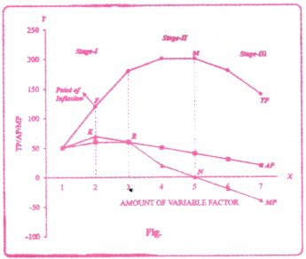
Diagram showing AP and MP curves.
Answer:

Question 7.
Second stage in the Law of variable proportions.
Answer:
Second stage : In this stage,

1. The Total Product (TP) curve increases at diminishing rate and reaches its maximum and constant at Point ‘M’ (Saturation Point).
2. The Average Product (AP) curve starts to fall after reaching its maximum (at AP = MP).
3. The Marginal Product (MP) curve continuously falls and becomes zero at the point of saturation i.e., at point ‘M’. (Here, the slope of Total product is zero at point ‘M’).
4. Second stage ends, where total product is at its maximum and marginal product is zero.
5. This stage is called the Law of Diminishing Returns.

Question 8.
Law of Supply.
Answer:
The law of supply explains the functional relationship between price of a commodity and its quantity supplied. “Other things remaining the same, as the price of a commodity rises, its supply is extended, and as the price falls, its supply is contracted”.

The quantity offered for sale varies directly with price i.e. the higher the price the larger is the supply and vice-versa.

Question 9.
Elasticity of Supply.
Answer:
The price elasticity of supply is the degree of responsiveness of quantity supplied to changes in the price of the good. More specifically, the price elasticity of supply, denoted by es, is defined as follows,

e_s = \(\frac{Percentage change in quantity supplied}{Percentage change in price}\)
= \(\frac{\frac{\Delta \mathrm{Q}}{\mathrm{Q}} \times 100}{\frac{\Delta \mathrm{P}}{\mathrm{P}} \times 100}\)
= \(\frac{\Delta \mathrm{Q}}{\Delta \mathrm{P}} \times \frac{\mathrm{P}}{\mathrm{Q}}\)
Where, ∆Q = Change in quantity of the good supplied;
∆P = Change in price,
P = Original price,
Q = Original quantity.

Note: The price elasticity of supply value ranges between 0 & ∞.

One Word Answer Questions

Answer the following questions in ONE WORD.

Question 1.
The responsiveness of quantity supplied due to change in price of a good is called:
Answer:
Elasticity of supply

Question 2.
The set of all possible combinations of two inputs that yield the same maximum possible level of output is known as :
Answer:
Isoquant

Question 3.
Which factor of production has been rightly defined as Produced means of production ?
Answer:
Capital

Question 4.
Under the law of variable proportions, at point of inflexion, marginal product is :
Answer:
Maximum

Question 5.
The economies that occurred to each member firm as a result of the expansion of the industry as a whole are known as …………….
Answer:
External economies

Fill in the blanks

Question 1.
When total product is 10 units and units of variable factor are 5, the average product will be ___________
Answer:
Units

Question 2.
When TP becomes constant at its maximum, MP is equal to ___________
Answer:
Zero (0)

Question 3.
When the supply curve shifts to right side, it is called ___________
Answer:
Increase in supply

Question 4.
In short-run when average product increases, marginal product is ___________
then average product.
Answer:
Greater then average product

Question 5.
When percentage change in output is greater than percentage change in inputs, it is called ___________
Answer:
Increasing returns to scale

Multiple Choice Questions

Question 1.
The Law of Variable Proportions when MP = AP, then AP is :
1) Maximum
2) Minimum
3) Negative
4) Zero
Answer:
1) Maximum

Question 2.
The behaviour of output due to change in all inputs is studied by :
1) The Law of Variable Proportions
2) The Law of Diminishing Returns
3) The Law of returns to scale
4) The law of returns to a factor
Answer:
3) The Law of returns to scale

Question 3.
In Cobb-Douglas production function, when a + b = 1, it exhibits.
1) Increasing return to scale
2) Constant return to scale
3) Decreasing return to scale
4) Negative return to scale
Answer:
2) Constant return to scale

Question 4.
Isoquant measures.
1) Marginal rate at technical situation between labour and capital
2) Marginal rate of substitution between two goods
3) Marginal utility of money
4) Marginal Efficiency of capital
Answer:
1) Marginal rate at technical situation between labour and capital

Question 5.
The stage of actual production in the law of returns to scale:
1) Increasing returns to scale
2) Constant returns to scale
3) Diminishing returns to scale
4) Negative returns to scale
Answer:
2) Constant returns to scale

AP Inter 1st Year Economics Study Material