Cost and Revenue Analysis Questions and Answers AP Inter 1st Year Economics Chapter 5

AP Inter 1st Year Economics 5th Lesson Cost and Revenue Analysis Questions and Answers

Essay Questions

Write an essay on the following questions.

Question 1.
Explain the different short-run cost structure of a firm.
Answer:
In the short run, a firm’s cost structure can be broken down into several key components. It is important to understand these different types of costs of analyze a firms profitability and decision-making. Here are the main short-run cost concepts.

1. Fixed Cost (FC):
These are costs that do not change with the level of output in the short run. They remain constant regardless of whether the firm produces a lot, a little, or even nothing at all. These are associated with the firm’s fixed factors of production, such as plant and equipment and contractual obligations.
Eg: Rent for building and land, salaries of permanent staff.

2. Variable Costs (VC) :
These are costs that change directly with the level of output. As the firm produces more, its variable costs increase, as it produces less they decrease. If the firm produces nothing, its variable costs are zero.
Eg: i) Cost of raw-materials.
ii) Wages of temporary (or) hourly workers.

3. Total Costs (TC):
This is the sum of all costs incurred by a firm in producing a certain level of output. It is the combination of total fixed costs and total variable costs.
TC = TFC + TVC
Since fixed costs remain constant in the short run, changes in total cost are solely driven by changes in variable costs as output levels fluctuate.

4. Average Fixed Costs (AFC) :
This is the fixed cost per unit of output. It is calculated by dividing total fixed cost by the quantity of output (Q).

The formula for Average Fixed Cost = AFC = \(\frac{FC}{Q}\). AFC decreases as output increases because the constant total fixed cost is spread over a larger number of units. This results in a downward sloping AFC curve.

5. Average Variable Cost (AVC) :
This is the variable cost per unit of output. It is calculated by dividing total variable cost by the quantity of output (Q).
The formula for Average Variable Cost = AVC = \(\frac{VC}{Q}\).

The AVC curve is typically U shaped. Intially, as output increases, AVC may fall due to increasing efficiency. However beyond a certain point, as variable factors become less productive (due to the law of diminishing returns) AVC starts to rise.

6. Average Total Cost or Average Cost (ATC or AC) :
This is the total cost per unit of output. It can be calculated in two ways:

• Dividing Total Cost by the quantity of output, ATC = \(\frac{TC}{Q}\).
• Adding Average Fixed Cost and Average Variable Cost.
  ATC = AFC + AVC

The ATC curve is also typically U-shaped. It reflects the combined influence of the falling AFC and the U-shaped AVC. ATC falls initially as AFC decreases rapidly, but eventually rises as the increase in AVC outweighs the decrease in AFC. The minimum point of the ATC curve represents the most efficient level of production in the short run.

7. Marginal Cost (MC) :
It is the additional cost incurred by producing one more unit of output. It measures the change in total cost resulting from a one-unit change in quantity. The formula for MC = \(\frac{\Delta \mathrm{TC}}{\Delta \mathrm{Q}}\).

Since fixed costs do not change with output, marginal cost is also equal to the change in total variable cost resulting from a one unit change in quantity.

MC = \(\frac{\Delta \mathrm{VC}}{\Delta \mathrm{Q}}\)

The MC curve is also typically U-shaped. It initially falls due to increasing marginal returns but eventually rises due to diminishing marginal returns. TheMC curve insects both the AVC and ATC curves at their minimum points.

Question 2.
Compare the relationship between AR and MR under perfect competition and imperfect competition.
Answer:
In Economic returns, the relationship between AR and MR varies significantly depending on the market structure specifically between perfect competition and imperfect competition.

Perfect Competition : In a perfectly competitive market, firms are price takers, meaning they have no control over the market price. The market price is determined by the interaction of supply and demand. Under these conditions ;

AR : The AR is equal to market price. This is because each unit sold fetches the same price, and thus, the total revenue divided by the number of units sold is the market price.

MR : The marginal revenue is also equal to the market price. This is because selling an additional unit does not affect the price, and the revenue from the additional unit is the same as the market price.
So, AR = MR = Price

Table : Revenue under Perfect Competition (in Rs.)
Output	Price	Total Revenue	Average Revenue	Marginal Revenue
1	10	10	10	10
2	10	20	10	10
3	10	30	10	10
4	10	40	10	10
5	10	50	10	10
6	10	60	10	10

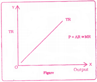
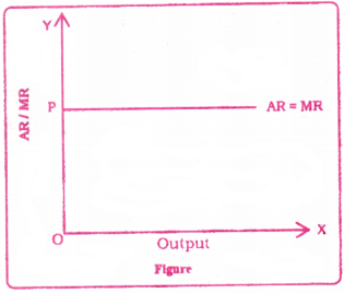
It is clear from the table and diagrams that the total revenue increases with an increase in quantity. When there is no change in price, average revenue remains the same. Marginal revenue is equal to the average revenue is fig. TR curve slopes upwards with a constant slope. Since, AR = MR it is the same curve which are horizontal and parallel to OX-axis. The AR curve is called Demand Curve.

Imperfect Competition : In Imperfect competition, which includes monopolistic competition and oligopoly, firms have some degree of market power and can influence the price of their products. This leads to a different relationship between AR and MR.

AR : The AR is the price at which the firm sells its products. However, to sell more units, the firm must lower its price, which affects the AR.

MR : The MR is less than the AR. This is because to sell an additional unit, the firm must lower the price on all units sold, not just the additional unit. Therefore, the revenue from the additional unit is less than the price of that unit.

MR < AR

Table (in Rs.)
Output	Price	Total Revenue	Average Revenue	Marginal Revenue
1	10	10	10	10
2	9	18	9	8
3	8	24	8	6
4	7	28	7	4
5	6	30	6	2
6	5	30	5	0
7	4	28	4	– 2
8	3	24	4	– 4

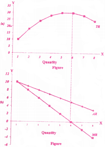
The table and diagrams (figures) reveals that as price falls, sales may improve and total revenue also increases gradually. Hence, the TR curve initially increases, reaches its maximum at a certain level of output and then falls after reaching its maximum. So that the shape of TR curve takes an “inverted U” shape. On the other hand, as the price falls, average revenue and marginal revenue decrease. Hence, the AR and MR curves slope, downwards and MR curve lies below the AR curve. It is to be noted that MR can be zero or even negative, but AR cannot be zero.

Relationship between TR and MR:

1. When TR increases MR falls.
2. When TR reaches its maximum (or) remains constant, MR becomes zero.
   (The slope of TR = 0).
3. When TR decreases, MR becomes negative.

Question 3.
Discuss the Long-run Cost Curves with a suitable diagram.
Answer:
Shape of Long run Cost Curves :

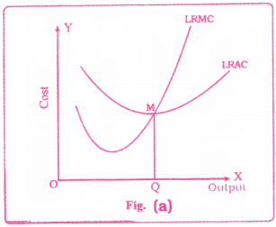
Let us check how the LRMC curve looks like. For the first unit of output, both LRMC and LRAC are the same. Then, as output increases, LRAC initially falls, and then, after a certain point, it rises. As long as average cost is falling, marginal cost must be less than the average cost. When the average cost is rising, marginal cost must be greater than the average cost. LRMC curve is a ‘U’-shaped curve. It cuts the LRAC curve from below at the minimum point of the LRAC. This is shown in Fig. (a)

Long-run average cost curve:

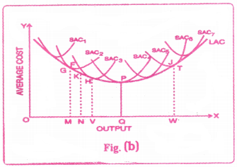
The long run average cost curve (LAC) is a smooth curve enveloping all short-run average cost curves (SACs). The LAC is drawn as tangent to each of the SACSs. The long run average cost curve (LAC) is called ‘planning curve’, ‘boat shaped curve’ and ‘envelope curve’. Whereas, the short- run average cost curves (SACs) are called ‘plant curves’.

When LAC is declining, it is tangent to the falling portions of SACs and when LAC is rising, it is tangent to the rising portions of SACs. Hence, the LAC is a “U” shaped curve. The behaviour of LAC depends upon the “Law of returns to scale” (fig.(b)).

Question 4.
Discuss the short-run Cost Curves with a suitable diagram.
Answer:
Short-run Total Costs – Graph :
These are, total fixed cost (TFC), total variable cost (TVC) and total cost (TC) curves for a firm. Total cost is the vertical sum of total fixed cost and total variable cost.

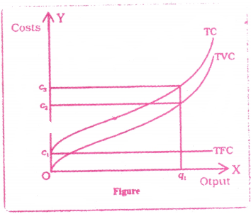
In the figure, output is measured on OX – axis and costs on OY-axis. Since total fixed cost remains constant at all levels of output in the short-run, TFC curve is a horizontal line and parallel to the OX-axis. On the other hand, TVC curve rises along with the level of output. It starts from origin and slopes upwards to the right. The sum of TC curve and TVC curve is rise with the level of output and slopes upwards to the right. TC and TVC curves are parallel to each other as the difference is the same (TFC).

Short run Average Costs :

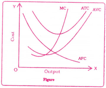
Fig. shows the average and marginal cost curves. It may be observed that AFC falls from downwards left to right continuously. The fall is steep in the beginning but flatter later. The AFC curve is convex to origin. This curve is a rectangular hyperbola. It is because at any point on the curve multiplication of the AFC by the number of output units gives fixed value.

Both ATC curve and the AVC curve fall upto a point and rise later. The curves are ‘U’-shaped cost curves. It may be observed that ATC curve is above the AVC curve and the distance between the two keeps declining. Because it represents the AFC which continuously declining, MC curve is also a U-shaped cost curve. It cuts both ATC and AVC from below at their minimum (lowest) points.

Short Answer Questions

Write the answers briefly for the following questions.

Question 1.
Briefly explain the various concepts of costs.
Answer:
The following are the various concepts of costs.

1. Explicit Costs : These are actual monetary payments made for resources like wages, rent and materials.
   Eg: Rent for the factory building
2. Implict Costs : Cost of using resources owned by the firm itself; without direct monetary payment.
   Eg : Owner’s time or capital.
3. Opportunity Cost : It is the cost of next best alternative, sacrificed in order to obtain that commodity. These are also called alternative cost.
4. Money Cost: The money outlays of a firm in the process of production of its output, in terms of money are called money costs.
   Eg. : Wages and salaries.
5. Real Cost : It is defined as the efforts and sacrifices producer has to make for producing a desired output.
6. Short run Costs : These refer to costs relating to the short period of time.
   Eg.: Capital equipment.
7. Long run Costs : These relating to the long period of time. All costs are variable in the long run.

Question 2.
Explain the relationship between Average Cost and Marginal Cost with the help of diagram.
Answer:
Relationship between Average cost and Marginal Cost :
The Average Cost (AC) is the cost per unit of output and the Marginal Cost (MC) is the total cost of producing an additional unit of output.

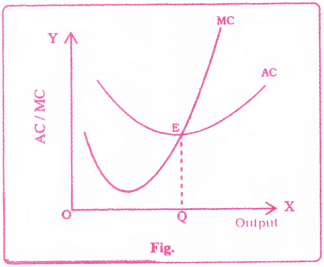
The average and marginal cost concepts are important to a producer in determining the optimum output. Both Average Cost (AC) and Marginal Costs (MC) are “U” shaped due to the operation of “the law of variable proportions”. The minimum point of Average Cost (AC) curve is called the “Optimum point”. At optimum point, Average Cost is equal to Marginal Cost (AC = MC). The output at optimum point is called “Optimum output”, shown in the figure.

From the graph it is clear that,

a) When AC is falling MC lies below the AC i.e., MC is less than AC (MC < AC). MC may be falling or rising in this condition.
b) When AC is minimum (constant) at point ‘E’, MC is equal to AC (MC = AC). This point called optimum point and OQ output is optimum output
c) When AC is rising beyond OQ level of output, MC is also rises and becomes greater than AC (MC > AC).

Question 3.
What is Revenue ? Explain different types of Revenues.
Answer:
Revenue : The amount of money that the producer receives in exchange for the goods (sale proceeds) is called producer’s receipts or revenue. In other words, the total sale proceeds of a firm is known as revenue. There are three types of revenue: i) Total Revenue, ii) Average Revenue, and iii) Marginal Revenue.

Total Revenue (TR) : Total amount of money or income received by the firm from the sale of a certain quantity of output is called total revenue. It is obtained by multiplying the price of a commodity by the number of units sold i.e. TR = P × Q.
P = Price of the good
Q = The quantity of the good sold.

Average Revenue (AR) : It is the revenue per unit of good sold. It is computed by dividing the total revenue by the number of units of a good sold.
AR = \(\frac{T R}{Q}\)
= \(\frac{P \times Q}{Q}\) = P
It is clear that the AR at each level of output is equal to the price per unit i.e. AR = P.

Marginal Revenue : It is the addition to the total revenue by selling one additional unit of the good i.e., the revenue which would be earned by selling an additional unit of the good.
MR = \(\frac{Change in TR}{Change in Quantity}\)
= \(\frac{\Delta \mathrm{TR}}{\Delta \mathrm{Q}}\)
MR_n = TR_n – TR_n-1

Question 4.
Explain the Revenue Curves in imperfect competition.
Answer:
MR < AR

Table (in Rs.)
Output	Price	Total Revenue	Average Revenue	Marginal Revenue
1	10	10	10	10
2	9	18	9	8
3	8	24	8	6
4	7	28	7	4
5	6	30	6	2
6	5	30	5	0
7	4	28	4	– 2
8	3	24	4	– 4

The table and diagrams (figures) reveals that as price falls, sales may improve and total revenue also increases gradually. Hence, the TR curve initially increases, reaches its maximum at a certain level of output and then falls after reaching its maximum. So that the shape of TR curve takes an ‘inverted U” shape. On the other hand, as the price falls, average revenue and marginal revenue decrease. Hence, the AR and MR curves slope downwards and MR curve lies below the AR curve. It is to be noted that MR can be zero or even negative, but AR cannot be zero.

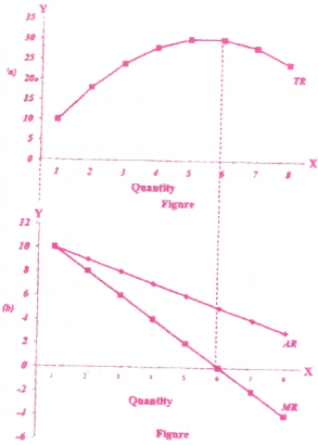
Relationship between TR and MR:

1. When TR increases MR falls.
2. When TR reaches its maximum (or) remains constant, MR becomes zero. (The slope of TR = 0).
3. When TR decreases, MR becomes negative.

Question 5.
The following table shows the total cost schedule of a firm. Calculate the TFC, TVC, AFC and AVC schedule of the time.

Q	TC
0	10
1	30
2	45
3	55
4	70
5	90
6	120

Answer:

Q	TC	TFC	TVC	AFC	AVC
0	10	10	0	0	–
1	30	10	20	10.00	20.00
2	45	10	35	5.00	17.50
3	55	10	45	3.30	15.00
4	70	10	60	2.50	15.00
5	90	10	80	2.00	16.00
6	120	10	110	1.65	18.33

Question 6.
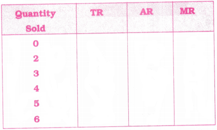
Compute the Total Revenue, Average Revenue and Marginal Revenue schedules in the following table. Market price of each unit of the good is Rs. 10%.

Answer:

Quantity Sold	TR (P.Q)	AR Price	MR = TRn – TRn-1
0	10 × 1 = 10	10	10 – 0 = 10
2	10 × 2 = 20	\(\frac{20}{2}\) = 10	20 – 10 = 10
3	10 × 3 = 30	\(\frac{30}{3}\) = 10	30 – 20 = 10
4	10 × 4 = 40	\(\frac{40}{4}\) = 10	40 – 30 = 10
5	10 × 5 = 50	\(\frac{50}{5}\) = 10	50 – 40 = 10
6	10 × 6 = 60	\(\frac{60}{6}\) = 10	60 – 50 = 10

Question 7.
The following table shows the total cost schedule of a firm. What is the total fixed cost schedule of this firm? Calculate the TVC, AFC, AVC, AC and MC schedules of the firm.

Q	TC
0	10
1	30
2	45
3	55
4	70
5	90
6	120

Answer:

Q	TC	TFC (TC at 0)	TVC (TC – TFC)	AFC = TFC ÷ Output	AVC = TVC ÷ Output	AC = TC ÷ Output	MC = TCn – TC n-1
0	10	10	0	–	–	–	–
1	30	10	20	10	20	30	20
2	45	10	35	5	17.50	22.5	15
3	55	10	45	3.33	15	18.33	10
4	70	10	60	2.50	15	17.50	15
5	90	10	80	2	16	18.00	20
6	120	10	110	1.67	18.33	20.00	30

Question 8.
The following table gives the total cost schedule of a firm. It is also given that the average fixed cost at 4 units of output is Rs.5. Find the AVC, AFC, AC and MC schedule of the firm for the corresponding values of output.

Q	TC
1	50
2	65
3	75
4	95
5	130
6	185

Answer:

Output	TC	TFC	TVC	SAC	AFC	AVC	SMC
1	50	20	30	50	20	30	30
2	65	20	45	32.50	10	22.50	15
3	75	20	55	25	6.67	18.33	10
4	95	20	75	23.75	5	18.75	20
5	130	20	110	26	4	22	35
6	185	20	165	30.83	3.33	27.50	55

Formulas :

1. TVC = TC – TFC
2. SAC (AC) = TC ÷ Output.
3. AVC = TVC ÷ Output
4. SMC_(n) (MC_n) = TC_n – TC_n-1
5. TFC = AFC × Unit of output = 5 × 4 = Rs.20
6. AFC = \(\frac{TFC}{Output}\)

Very Short Answer Questions

Question 1.
Explicit Cost.
Answer:
The remuneration paid to outside factors of production is called explicit costs. They involve cash payments and are recorded in the books of accounts. Explicit costs are also called “Accounting costs”.
Eg.: Wages to the labourers, rent for the factory building, payments for raw materials, etc.
Both economists and accountants take them into account.

Question 2.
Implicit Cost.
Answer:
The cost of factors owned by the entrepreneur himself and employed in his own business is called implicit costs. These are also called as imputed costs.
Eg : Rent of own factory building, interest on own money, capital investment Economists take into account implied costs also while accountants ignore them, because no monetary transactions takes place.

Explicit Cost + Implicit cost = Total Cost

Question 3.
Opportunity Cost.
Answer:
Opportunity Cost is the cost of next best alternative, sacrificed in order to obtain that commodity.

It is a loss of income due to opportunity foregone. Opportunity cost is also called ‘alternative cost’. It arises because of scarcity and alternative uses of resources.

Question 4.
Enveloping curve.
Answer:
Long-run average cost curve:

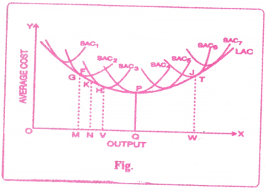
The long run average cost curve (LAC) is a smooth curve enveloping all short-run average cost curves (SACs). The LAC is drawn as tangent to each of the SACs. The long run average cost curve (LAC) is called ‘planning curve’, ‘boat shaped curve’ and ‘envelope curve’. Whereas, the short-run average cost curves (SACs) are called ‘plant curves’.

When LAC is declining, it is tangent to the falling portions of SACs and when LAC is rising, it is tangent to the rising portions of SACs. Hence, the LAC is a “U” shaped curve. The behaviour of LAC depends upon the “Law of returns to scale” (fig-(b))

Question 5.
Diagram showing AC and MC.
Answer:

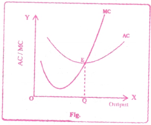
a) When AC is falling MC lies below the AC i.e., MC is less than AC (MC < AC). MC may be falling or rising in this condition.
b) When AC is minimum (constant) at point ‘E’, MC is equal to AC (MC = AC). This point called optimum point and OQ output is optimum output.
c) When AC is rising beyond OQ level of output, MC is also rises and becomes greater than AC (MC > AC).

Question 6.
Horizontal Revenue Curve.
Answer:
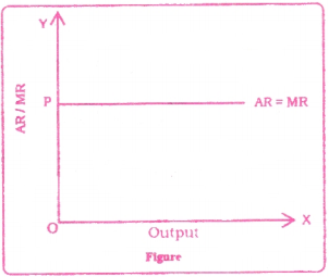
We have seen that a perfectly competitive firm’s marginal revenue curve is simply a horizontal line at the market price and that this same line is also the firm’s average revenue curve.

For the perfectly competitive firm,
MR = P = AR.

Question 7.
Sloping AR, MR Curves Text.
Answer:
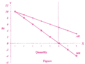
As the price falls, AR and MR decrease. Hence the AR and MR curves slope downwards and MR curve lies below the AR curve. It is to be noted that MR can be zero or even negative, but AR can not be zero.

Question 8.
The following table shows the total revenue and total cost schedules of a competitive firm. Calculate the profit at each level output.
Answer:

Quantity sold	TR (Rs.)	TC (Rs.)	Profit (TR – TC) Rs.
0	0	5	(0 – 5) = – 5
1	5	7	(5 – 7) = – 2
2	10	10	(10 – 10) = 0
3	15	12	(15 – 12) = 3
4	20	15	(20 – 15) = 5
5	25	23	(25 – 23) = 2
6	30	33	(30 – 33) = – 3
7	35	40	(35 – 40) = – 5

Question 9.
From the following details, find out the Average Variable Cost of 10 units.

Output (Units)	Total Cost (in Rs.)
0	100
5	200
10	400
15	600

Answer:
AVC = \(\frac{TVC}{Q}\)
Total Cost for 0 units =100 Rs.
Total Cost for 10 units = 400 Rs.
TVC = TC – TVC = 400 – 100 = 300
AVC = \(\frac{300}{10}\) = 30
∴ The Average Variable Cost AVC for 10 units is Rs. 30 per unit.

Question 10.
What is the Average total cost in producing 20 units ? If fixed cost is Rs. 1000/- and average variable cost is Rs. 2 ?
Answer:
Fixed Cost = 1,000 Rs.
AVC = Rs. 2
Quantity = 20 units
TVC = AVC × Q
= 2 × 20 = 40

TC = FC + TVC
= 1000 + 40 = 1040
∴ The Average total cost in producing 20 units is Rupees 52 per unit.

One Word Answer Questions

A) Answer the following question in ONE WORD.

Question 1.
Mr. Sreenu is working as a manager in his own factory. Which concept of cost covers the salary of Mr. Sreenu?
Answer:
Implicit cost

Question 2.
The Average Cost (AC) minus Average Fixed Cost (AFC) equals to:
Answer:
Average Variable Cost (AVC)

Question 3.
If after selling 10 units the total revenue is Rs. 10,000 and after selling 12 units the total revenue increases to Rs. 15,000- then marginal revenue is:
Answer:
Rs. 2,500

Question 4.
The Average Revenue (\(\frac{TR}{Q}\)) is always equals to:
Answer:
Price

Question 5.
The mathematical relation between cost of a product and the various determinants of cost is known as:
Answer:
Cost function

Fill in the blanks

Question 1.
The cost incurred by producing an additional unit of output is ___________.
Answer:
Marginal Cost

Question 2.
The Long-run Average Cost (LAC) curve is also called as ___________.
Answer:
Envelope curve

Question 3.
The shape of average fixed cost curve is ___________.
Answer:
Rectangular hyperbola

Question 4.
When the average cost is at its minimum, then the marginal cost is ___________.
Answer:
Equal to average cost

Question 5.
When the average revenue decreases, then the marginal revenue is ___________.
Answer:
Less than average revenue

Multiple Choice Questions

Question 1.
The costs of self-owned and self-employed resources are termed as:
1) Accounting cost
2) Explicit cost
3) Money cost
4) Implicit cost
Answer:
4) Implicit cost

Question 2.
Find the total cost, when TFC = Rs. 200/- and TVC = Rs.225 :
1) Rs. 200
2) Rs.225
3) Rs.425
4) Rs.25
Answer:
3) Rs.425

Question 3.
If the total cost at 5 units of output is Rs.5007 and at 7 units, it is Rs. 7007. Find the marginal cost at 7th unit (In Rs.)?
1) 400
2) 300
3) 200
4) 100
Answer:
4) 100

Question 4.
The Total Cost (TC) at zero (0) units of output is:
1) Equal to zero
2) Equal to total fixed cost
3) Equal to total variable cost
4) Equal to marginal cost
Answer:
2) Equal to total fixed cost

Question 5.
The minimum point of the Average Cost (AC) curve is known as:
1) Equilibrium point
2) Break Even Point (BEP)
3) Point of inflexion
4) Optimum point
Answer:
4) Optimum point

AP Inter 1st Year Economics Study Material